Predictions From Data Frames

Introduction

In many experimental designs, model parameters vary across conditions or subjects and are conveniently stored in tabular (i.e., spreadsheet) form. In most cases, this kind of information is loaded into R as a data frame. This vignette demonstrates how to use a data frame to generate multiple predictions quickly.

We will walk through the full process using the package’s included subopt_avian data set as an example.

The `subopt_avian` Data Set

Dunn et al. (2024) compiled the results of an extensive collection of studies investigating suboptimal choice behaviour. This dataset is included in the SiGN package.

The full data set is available as subopt_full. For model evaluation purposes, however, Dunn et al. (2024) focused on a curated subset of studies involving pigeons and starlings—particularly pigeons, which were the most extensively studied and yielded the most robust, consistently replicated findings. This filtered dataset is provided as subopt_avian.

Each row in subopt_avian corresponds to a unique study condition. Many of its columns—specifically columns 9 through 24—map directly to the parameters expected by the SiGN() model function (see the subopt_avian documentation for full details on the column structure).

library(SiGN)

# Display column names
names(subopt_avian)
#>  [1] "row"             "study"           "year"            "species"        
#>  [5] "exp"             "condition"       "n"               "cp"             
#>  [9] "il_dur_a"        "il_dur_b"        "tl_dur_a1"       "tl_dur_a2"      
#> [13] "tl_dur_b1"       "tl_dur_b2"       "tl_p_a1"         "tl_p_a2"        
#> [17] "tl_p_b1"         "tl_p_b2"         "tr_p_a1"         "tr_p_a2"        
#> [21] "tr_p_b1"         "tr_p_b2"         "il_sched_a"      "il_sched_b"     
#> [25] "tl_sched_a1"     "tl_sched_a2"     "tl_sched_b1"     "tl_sched_b2"    
#> [29] "forced_exposure" "DOI"             "ref"             "data_version"

Of special note is column 8 ($cp), which contains the observed choice proportion reported for each condition. These values can be directly compared to the choice proportions predicted by the SiGN model, which we will generate shortly.

Generating a List of Model Parameters

As detailed in the Get Started, to generate model predictions with the SiGN() function, we first need to prepare a list of model parameters in the format it expects.

These parameters are currently stored as columns in the subopt_avian data frame (specifically, columns 9 through 24). However, they are not yet in list form, and some required inputs—such as s_delta, beta_log, and beta_toggle—are not included in the data set. While these defaults are not parameters most users need to adjust, they must be present for SiGN() to run properly.

Rather than constructing this list manually, we use the choice_params() function. This function not only formats the input correctly but also performs important validation checks to ensure that all required arguments are present and well-formed.

To convert the relevant columns into a list of named arguments, we use do.call() in combination with as.list(). This allows us to pass the data frame columns directly into choice_params() as if we had typed them out individually.

# Store Model Parameters
#-------------------------------------------------------------------------------
# Extract relevant parameter columns (cols 9–24 align with choice_params())
data_cols <- subopt_avian[9:24]

# Construct model input list
params <- do.call(choice_params, as.list(data_cols))

The do.call() function dynamically calls choice_params() by unpacking the data frame columns into named arguments. In other words, do.call(choice_params, as.list(data_cols)) transforms each column into an argument like il_dur_a = ..., il_dur_b = ..., and so on—matching exactly what choice_params() expects. This only works because the column names in subopt_avian[9:24] are aligned with the argument names that choice_params() requires.

Generating the Predictions

Now that we have constructed a valid list of model parameters, we can pass it to the SiGN() function to generate predictions. This function returns a variety of outputs, but here we are specifically interested in the predicted choice proportions.

# Generate model predictions
#-------------------------------------------------------------------------------
preds <- SiGN(params)

The SiGN model’s predicted choice proportion, for each row of subopt_avian[9:24], can be called with preds$cp. These values can be compared directly to the observed choice proportions stored in subopt_avian$cp. For more information about the SiGN() function and its outputs, see the Get Started article.

Visualising the Predictions

To help visualise the model’s performance, we shall fit a simple linear regression to the observed versus predicted choice proportions. This provides a clear visual summary of their relationship and allows us to overlay both a fitted regression line and a 1:1 reference line. The closer the data points fall to the 1:1 line, the more closely the model’s predictions match the observed values—offering a quick and intuitive check on model accuracy.

# Fit a linear model comparing observed vs predicted
reg <- lm(subopt_avian$cp ~ preds$cp)

# Format annotation for plot
reg_txt <- sprintf(
  "y = %.2f + %.2f x\n",
  reg$coefficients[1], reg$coefficients[2]
)

library(ggplot2)

ggplot(mapping = aes(x = preds$cp, y = subopt_avian$cp)) +

  # Add 1:1 reference line (dashed) to assess prediction accuracy
  geom_abline(intercept = 0, slope = 1, linetype = 3) +

  # Plot each observed vs. predicted data point as an open circle
  geom_point(pch = 1, size = 1.75, stroke = 0.5) +

  # Fit and overlay a linear regression line (no confidence band)
  geom_smooth(method = "lm", se = FALSE) +

  # Axis labels
  labs(x = "Predicted", y = "Obtained") +

  # Add regression summary text
  annotate("text", x = 0.2, y = 0.9, label = reg_txt, size = 3.5) +

  # Base theme
  theme_bw(base_size = 12) +

  # Make axis text black for visibility
  theme(axis.text = element_text(colour = "black"))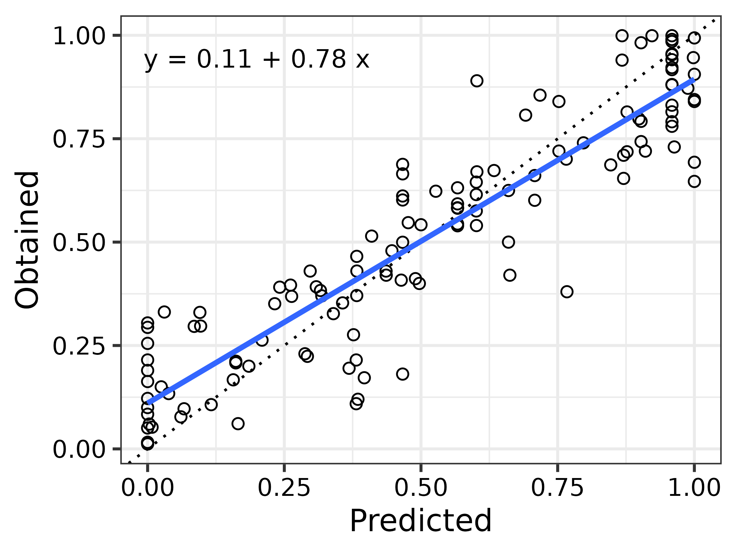

References

Dunn, R. M., Pisklak, J. M., McDevitt, M. A., & Spetch, M. L. (2024). Suboptimal choice: A review and quantification of the signal for good news (SiGN) model. Psychological Review. 131(1), 58-78. https://doi.org/10.1037/rev0000416